
1. Toolchain Overview
2026-06 Toolchain v0.33.1
1.1. Introduction
KDP toolchain is a set of software which provide inputs and simulate the operation in the hardware KDP 520, 720, 530, 630 and 730. For better environment compatibility, we provide a docker which include all the dependencies as well as the toolchain software.
In this document, you'll learn:
- What tools are in the toolchain.
- How to deploy the latest toolchain.
- How to utilize the tools through Python API.
Major changes of the current version
- [v0.33.1]
- Improve LayerNorm decomposition performance.
- Improve handling for models that reuse weights across multiple operators.
- Improve constant folding reliability.
- Improve example scripts for easy platform switching.
- Support ReduceMean fusion when
keepdimsis set to 0.
- [v0.33.0]
- Update TopK and Split node support.
- Improve per-channel radix handling for Mul nodes.
- Add warnings for models that may be sensitive to large value ranges or Sigmoid quantization.
- Fix Clip handling when the maximum value is set to
FLT_MAX. - Fix Slice and Concat handling for additional slicing patterns.
- Fix KL730 CPU execution for Mod nodes with constant inputs.
- Add a ktc warning for workflows with multiple BIE inputs.
- Add license information to kneronnxopt.
- Minor bug fixes.
1.2. Workflow Overview
In the following parts of this page, you can go through the basic toolchain working process to get familiar with the toolchain.
Below is a brief diagram showing the workflow of how to generate the binary from a floating-point model using the toolchain.
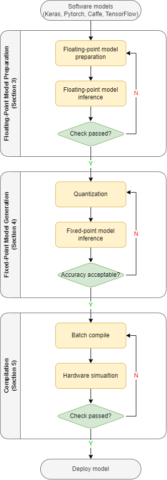
Figure 1. Diagram of working flow
To keep the diagram as clear as possible, some details are omitted. But it is enough to show the general structure. There are three main sections:
- Floating-point model preparation. Convert the model from different platforms to onnx and optimize the onnx file. Evaluate the onnx the model to check the operator support and the estimate performance. Then, test the onnx model and compare the result with the source.
- Fixed-point model generation. Quantize the floating-point model and generate bie file. Test the bie file and compare the result with the previous step.
- Compilation. Batch compile multiple bie models into a nef format binary file. Test the nef file and compare the result with the previous step.
In the following parts, we will use MobileNet V2 as the example. Details will be explained later in other sections.
And all the code below in this section can be found inside the docker at /workspace/examples/mobilenetv2/python_api_workflow.py.
The script accepts an optional platform argument. The default platform is 720, and supported values are 520, 530, 630, 720 and 730.
python python_api_workflow.py
python python_api_workflow.py 730
1.3. Toolchain Docker Deployment
We provide docker images for ease of deployment. Below are command for downloading and running the latest docker image.
# Pull the latest toolchain docker image.
docker pull kneron/toolchain:latest

# Login to the docker and mount host machine /mnt/docker into the docker at /docker_mount.
docker run --rm -it -v /mnt/docker:/docker_mount kneron/toolchain:latest
To learn more about the docker installation, docker image version management, docker usage and environment inside the docker, please check 2. Toolchain Deployment.
1.4. Floating-Point Model Preparation
Our toolchain utilities take ONNX files as inputs. This part of workflow is mainly about convert models from other platforms to ONNX and prepare the onnx for the quantization and compilation. There are three main steps: conversion, evaluation and testing.
For more details about the model conversion and optimization, please check 3. Floating-Point Model Preparation.
1.4.1. Model Conversion And Optimization
Before we start, we need to import our python package. The package name is ktc. You can simply start by having import ktc in the script.
In the following sections, we'll introduce the API and their usage. You can also find the usage using the python help() function.
Note that this package is only available in the docker due to the dependency issue.
Here the MobileNet V2 model is already in ONNX format. So, we only need to optimize the ONNX model to fit our toolchain. The following model optimization code is in Python since we are using the Python API.
import onnx
# Import the ktc package which is our Python API.
import ktc
# Import the onnx optimizer which is used to optimize the onnx model.
import kneronnxopt

# Load the model.
original_m = onnx.load("/workspace/examples/mobilenetv2/mobilenetv2_zeroq.origin.onnx")
# Optimize the model using optimizer for onnx model.
optimized_m = kneronnxopt.optimize(original_m)
# Save the onnx object optimized_m to path /data1/optimized.onnx.
onnx.save(optimized_m, '/data1/optimized.onnx')
1.4.2. Model Evaluation
Before we start quantizing the model and try simulating the model, we need to test if the model can be taken by the toolchain structure and estimate the performance. IP evaluator is such a tool which can estimate the performance of your model and check if there is any operator or structure not supported by our toolchain.
platform = "720"
# Create a ModelConfig object. For details about this class, please check Appendix Python API.
# Here we set the model ID to 32769, the version to 8b28 and the target platform.
# The `optimized_m` is from the previous code block.
km = ktc.ModelConfig(32769, "8b28", platform, onnx_model=optimized_m)

# Evaluate the model. The evaluation result is saved as string into `eval_result`.
eval_result = km.evaluate()
The evaluation result will be returned as string. User can also find the evaluation result under /data1/kneron_flow/.
The report is in html format: model_fx_report.html. You can check the report in command line with:
w3m /data1/kneron_flow/model_fx_report.html1.4.3. Floating-Point Model Inference
Before going into the next section of quantization, we need to ensure the optimized onnx file can produce the same result as the originally designed model. Here we introduce the E2E simulator which is the abbreviation for end to end simulator. It can inference a model and simulate the calculation of the hardware. We are using the onnx as the input model now. But it also can take other file formats which would be introduced later.
Since toolchain v0.21.0, we take inputs with exactly the same shape as onnx instead of the previous channel last format.
Since toolchain v0.22.0, we provide ktc.convert_channel_last_to_first to help converting channel last inputs to channel first(image only). For details, please check 3. Floating-Point Model Preparation
# Import necessary libraries for image processing.
from PIL import Image
import numpy as np

# A very simple preprocess function. Note that the image should be in the same format as the ONNX input (usually NCHW).
def preprocess(input_file):
    image = Image.open(input_file)
    image = image.convert("RGB")
    img_data = np.array(image.resize((224, 224), Image.BILINEAR)) / 255
    img_data = np.transpose(img_data, (2, 0, 1))
    # Expand 3x224x224 to 1x3x224x224 which is the shape of ONNX input.
    img_data = np.expand_dims(img_data, 0)
    return img_data

# Use the previous function to preprocess an example image as the input.
input_data = [preprocess("/workspace/examples/mobilenetv2/images/000007.jpg")]

# The `onnx_file` is generated and saved in the previous code block.
# The `input_names` are the input names of the model.
# The `input_data` order should be kept corresponding to the input names. It should be in the same shape as ONNX (NCHW).
# The inference result will be save as a list of array.
floating_point_inf_results = ktc.kneron_inference(input_data, onnx_file='/data1/optimized.onnx', input_names=["images"])
After getting the floating_point_inf_results and post-process it, you may want to compare the result with the one generated by the source model.
Since we want to keep this flow as clear as possible in this walk through, we do not provide any postprocess and skip the step of comparing the inference result for this example.
1.5. Fixed-Point Model Generation
In this chapter, we would go through fixed-point model generation and verification. In our toolchain, the fixed-point model is generated by quantization and saved in bie format. It is encrypted and not available for visualization. The details about the fixed-point model generation are under 4. Fixed-Point Model Generation.
1.5.1. Quantization
Quantization is the step where the floating-point weight are quantized into fixed-point to reduce the size and the calculation complexity.
The Python API for this step is called analysis. It is also a class function of ktc.ModelConfig.
This is a very simple example usage. There are many more parameters for fine-tuning. Please check 4. Fixed-Point Model Generation.
# Preprocess images as the quantization inputs. The preprocess function is defined in the previous section.
import os
raw_images = os.listdir("/workspace/examples/mobilenetv2/images")
input_images = [preprocess("/workspace/examples/mobilenetv2/images/" + image_name) for image_name in raw_images]

# We need to prepare a dictionary, which mapping the input name to a list of preprocessed arrays.
input_mapping = {"images": input_images}

# Quantization the model. `km` is the ModelConfig object defined in the previous section.
# For more fine-tuning arguments, please check '4. Fixed-Point Model Generation'.
# The quantized model is saved as a bie file. The path to the bie file is returned as a string.
# It also generates a html report with more details. Please check `/data1/kneron_flow/model_fx_report.html`
bie_path = km.analysis(input_mapping, threads = 4)
1.5.2. Fixed-Point Model Inference
Before going into the next section of compilation, we need to ensure the quantized model do not lose too much precision.
We would use ktc.kneron_inference here, too. But here we are using the generated bie file as the input.
The python code would be like:
# Use the previous function to preprocess an example image as the input.
# Here the input image is the same as in section 1.4.3.
input_data = [preprocess("/workspace/examples/mobilenetv2/images/000007.jpg")]

# Inference with a bie file. `bie_path` is defined in section 1.5.1.
fixed_point_inf_results = ktc.kneron_inference(input_data, bie_file=bie_path, input_names=["images"], platform=int(platform))

# Compare `fixed_point_inf_results` and `floating_point_inf_results` to check the precision loss.
As mentioned above, we do not provide any postprocess. In reality, you may want to have your own postprocess function in Python, too.
After getting the fixed_point_inf_results and post-process it, you may want to compare the result with the floating_point_inf_results
which is generated in section 1.4.3 to see if the precision lose too much. We skip this step to keep this quick start as simple as possible.
1.6. Compilation
Finally, we can compiling models into the binary files which are in nef format. In fact, our compiler can compile multiple models into just one nef file, that's why it is called 'batch compile'. However in this simple example, we would not go that deep. If you are willing to learn more, please check 5. Compilation.
1.6.1. Batch Compile
Batch compile turns multiple models into a single binary file. But, we would use the single model we just generated for now.
# `compile` function takes a list of ModelConfig object.
# The `km` here is first defined in section 3 and quantized in section 4.
# The compiled binary file is saved in nef format. The path is returned as a `str` object.
nef_path = ktc.compile([km])
1.6.2. Hardware Simulation
After compilation, we need to check if the nef can work as expected.
We would use ktc.kneron_inference here again. And we are using the generated nef file this time.
# `nef_path` is defined in section 1.6.1.
binary_inf_results = ktc.kneron_inference(input_data, nef_file=nef_path, platform=int(platform), input_names=["images"])

# Compare binary_inf_results and fixed_point_inf_results. They should be almost the same.
After getting the binary_inf_results and post-process it, you may want to compare the result with the fixed_point_inf时_results which is generated in section 1.5.2 to see if the results match. Once the results match, then you can deploy your model onto the chip. Congratulations.
1.7 What's Next
This overview section only provides a simplified version of the workflow. The aim of this section is to get your an idea of how our toolchain shall be utilized. There are much more details which help you deploy your own model and may greatly improve your model performance on-chip waiting in other section. Please check.
- 2. Toolchain Deployment
- 3. Floating-Point Model Preparation
- 4. Fixed-Point Model Generation
- 5. Compilation
There are also other useful tools and information:
- End to End Simulator: manual for the E2E simulator.
- Hardware Performance: common model performance table for Kneron hardwares and the supported operator list.
- Hardware Supported Operators: operators supported by the hardware.
- How to Interpret Fixed-Point Report: manual for interpreting the fixed-point report.
- Kneronnxopt: manual for the a more flexible onnx optimizer tool.
- ONNX Converters: manual for the script usage of our converter tools. This tool is only for ONNX opset 11/12.
- Quantization 1 - Introduction to Post-training Quantization: introduction for the quantization.
- Quantization 2 - Post-training Quantization(PTQ) Flow and Steps: manual for the quantization flow and steps.
- Script Tools: manual for deprecated command line tools. Kept for compatibility of toolchain before v0.15.0)
- Toolchain History: manuals for history version of toolchain and the change log.
- Web GUI: a simple web interface for the toolchain docker image.
- YOLO Example: a step-by-step walk through using YOLOv3 as the example.
- Yolo Example (With In-Model Preprocess): a step-by-step walk through using YOLOv3 with in-model preprocess as the example.